


 4 / 16

I.K. Marchevsky, V.V. Puzikova
22
ISSN 1812-3368. Вестник МГТУ им. Н.Э. Баумана. Сер. Естественные науки. 2017. № 5
τ
.
t
t
xy
u v
y x
(5)
Here
t
xx
and
t
yy
are normal Reynolds or subgrid stresses and
t
xy
is shear Reynolds
or subgrid stress. In cases of algebraic turbulence models or models with one
differential equation the turbulent kinetic energy is assumed to be zero and only eddy
viscosity value is computed. For example, in the Smagorinsky model [8] the eddy
viscosity is defined by the following formula:
2
2
2
2
= ( ) 2
.
t
S
u
v
u v
C
x
y
y x
(6)
Here
S
C
is the empirical constant (the Smagorinsky constant). Choice of the
S
C
value
depends on the numerical method used to solve the problem, because at LES approach
the accuracy of large-scale vortex structures resolution depends not only on the mesh,
but also on numerical method properties, in particular, numerical dissipation. If the
numerical dissipation is large, it is necessary to choose smaller values of
,
S
C
and if
numerical dissipation is small, the
S
C
value should be chosen larger.
For EVM with differential equations the governing equations, initial and
boundary conditions are given by the turbulence model. In the most general way, they
may be written as the following:
0
1 2 3
4
( ) = Prod Dis
[(
) ] Add;
( , 0) = ( ),
|
= ,
| = ,
= 0.
ib
K
t
v
r
r
n
(7)
Here
Prod
is the production term which describes the generation of Reynolds or
subgrid stresses;
Dis
is the destruction term;
Add
is the additional term;
and
are given by the particular turbulence model (Table 2).
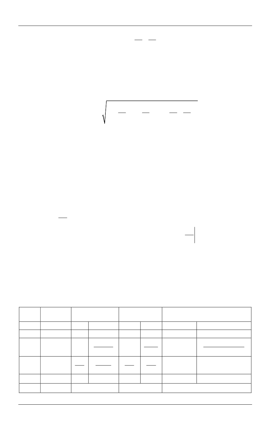
Table 2
Itemization of symbols in (7) and rules for
t
computation for some turbulence
models [3]
Term
Spalart —
Allmaras
k
k
k
SST
k
k
k
Add
0
0
0
0
0
0
1
(1 )
k
F D
Prod
P
P
1.44
P
k
P
5
9
P
k
P
1
(0.44 0.11 )
t
F P
Dis
D
3/2
turb
k
l
2
1.92
k
3/2
turb
k
l
2
3
40
3/2
/
turb
k l
1
0.0828 0.0078
F
t
/1.3
t
/ 2
t
/ 2
t
1
(1 0.5 )
t
F
1
(0.856 0.356 )
t
F
t
1
f
2
0.09 /
k
/
k
1
0.31 /
k G