


 3 / 16

Modification of the LS-STAG Immersed Boundary Method for Simulating Turbulent Flows
ISSN 1812-3368. Вестник МГТУ им. Н.Э. Баумана. Сер. Естественные науки. 2017. № 5
21
We denote the airfoil boundary as
.
K
Then the boundary conditions are the
following:
1 2 3
4
|
= ,
= 0,
| = .
ib
K
v
v
v
v v
n
It is possible to distinguish the linear turbulence scale
= ( )
turb turb
l
l
r
for all
turbulence models. In the framework of RANS approach this scale
turb
l
is equal to
scale
= ( ),
RANS RANS
l
l
r
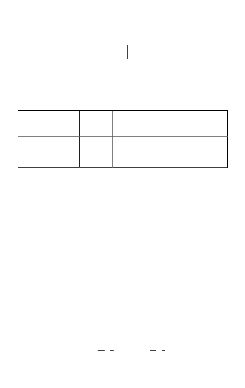
which is determined by the turbulence model (Table 1).
Table 1
Turbulence scale
RANS
l
for some turbulence models [3]
Turbulence model
RANS
l
Comments
Spalart — Allmaras [4]
w
d
w
d
is the distance between the field point and
the nearest wall
k
[5]
3/2 1
k
is the dissipation rate of the turbulent kinetic
energy
k
k
[6],
k
SST [7]
1/2 *
1
( )
k
is the specific dissipation rate of the
k
,
*
0.09
In case of LES approach, the scale
turb
l
is equal to subgrid scale:
= .
LES
LES
l
C
(2)
Here
= ( )
r
is the characteristic filter size at the point of computational domain
with the radius vector
,
r
and
LES
C
is the empirical constant, which choice depends
on the turbulence model and numerical method used to solve the problem (1) in the
whole. Within the DES approach the linear turbulence scale
turb
l
is equal to hybrid
linear scale
=min{
,
}.
DES
RANS DES
l
l
C
(3)
Here
DES
C
is the empirical constant similar to
,
LES
C
and the maximum of the mesh
steps at the point of computational domain with the radius vector
r
is used as the
characteristic filter size
= ( ).
r
Thus, DES operates as RANS in the domain where
the mesh is too coarse and not suitable for resolving turbulent structures, i. e. at
> ,
DES
RANS
C l
and DES operates as subgrid model for LES in the domain where the
grid is sufficiently fine [3]. It should be noted that Smagorinsky model is used only
within LES approach.
In this paper Eddy Viscosity turbulence models (EVM) are considered. In EVM
models the eddy viscosity
t
(and the turbulent kinetic energy
k
in case of two-
equation models) is simulated and Reynolds or subgrid stresses are evaluated using
the Boussinesq eddy viscosity assumption [3]:
2
2
= 2
;
= 2
;
3
3
t
t
t
t
xx
yy
u
v
k
k
x
y
(4)