


 12 / 16

I.K. Marchevsky, V.V. Puzikova
30
ISSN 1812-3368. Вестник МГТУ им. Н.Э. Баумана. Сер. Естественные науки. 2017. № 5
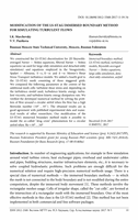
Flow simulation at low Reynolds numbers
(
3
Re <10
)
.
The LS-STAG method
allows to receive the results are in good agreement with the experimental and
computational data, even on very coarse meshes (Table 3). No turbulence models
have been used.
Table 3
Comparison of
D
C
and St at
Re =100
and
Re = 200
with known experimental
and numerical results from the literature
Source
Re 100
=
Re 200
=
D
C
St
D
C
St
Zdravkovich [10] (experiment)
1.21…1.41
0.16…0.17
–
–
LS-STAG (present study,
120 148)
1.31
0.17
1.33
0.20
LS-STAG (present study,
240 204)
1.32
0.17
1.33
0.20
LS-STAG (present study,
480 408)
1.32
0.17
1.33
0.20
Cheny [2] (LS-STAG,
550 350)
1.32
0.17
1.33
0.20
Henderson [11]
1.35
0.16
1.34
0.20
He [12]
1.35
0.17
1.36
0.20
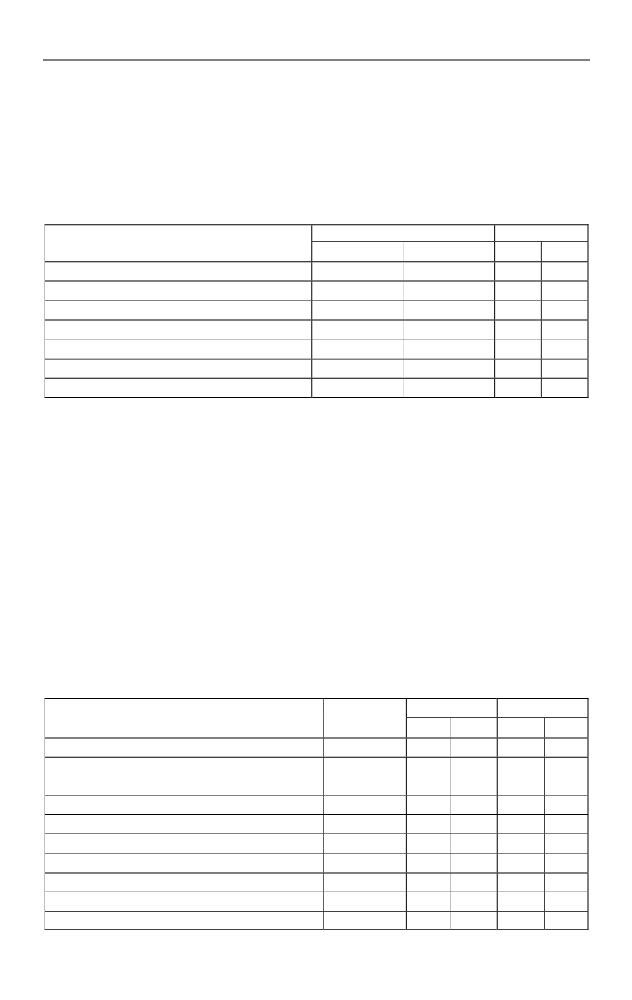
Flow simulation at medium Reynolds numbers
(
3
4
Re =10 10
)
.
The flow was
simulated at the Reynolds numbers
Re =1000
(on non-uniform meshes 120 148
with
2
=5 10
t
and 240 296
with
3
=10
t
) and
Re = 3900
(on non-uniform meshes
120 148
with
3
=10
t
and 240 296
with
4
= 5 10
t
). These values of the
Re
were
chosen because the experimental data [10, 11] and results of other researchers [14–17] are
known for them. Computational results are shown in Table 4 and in Fig. 5. These results
are in good agreement with experimental data for simulation on coarse meshes by using
the proposed modification of the LS-STAG method. But since the considered models
works well only at high Reynolds numbers, it is hardly possible to improve the numerical
results, for example, by mesh refinement. In our opinion the wall functions usage can be
an efficient solution to this problem.
Table 4
Comparison of
D
C
and
St
values with known experimental and numerical results
Turbulence model
Number
of cells
Re 1000
=
Re 3900
=
D
C
St
D
C
St
Experiment [10]
−
0.98
0.21
0.93
0.22
Experiment [13]
−
1.12
–
1.01
–
Smag., LES,
C
S
= 0.1 [14]
1 103 520
–
–
1.08
–
Smag., LES,
C
S
= 0.1 (spectral) [15]
30 720
–
–
1.01
0.22
Smag., LES,
C
S
= 0.1 (finite volume) [15]
855 040
–
–
1.07
0.24
,
k
RANS [16]
46 304
1.00
0.15
1.00
0.15
Real
,
k
RANS [16]
46 304
–
0.17
–
0.20
k
SST, RANS [16]
46 304
–
0.23
–
0.25
,
k
RANS [17], ANSYS
388 550
1.12
–
0.74
–
k
SST, RANS [17], ANSYS
388 550
0.99
–
0.62
–