


 9 / 17

S. Persheyev, D.A. Rogatkin
86
ISSN 1812-3368. Вестник МГТУ им. Н.Э. Баумана. Сер. Естественные науки. 2017. № 5
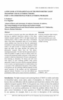
Fig. 5.
Schematic representation of the
1D medium with
N
inhomogeneities
r
i
inside it
In next figures, we will not draw black dots to indicate inhomogeneities. We will
simply denote their coordinates by short lines crossing the
X
-axis.
Single scattering approximation.
The simplest case of the pure scattering model is
the single scattering approximation (SSA). It gives the simplest solution of the 1D
scattering problem. SSA assumes scattering (more exactly — the back reflection in the
1D case) for the forward flus
F
+
(
x
)
on each inhomogeneity (decrement of
F
+
(
x
)
after
passing the inhomogeneity) and the absence of scattering for the backward flux
F
−
(
x
)
,
i. e. it assumes the negligible re-reflection process between any two heterogeneities
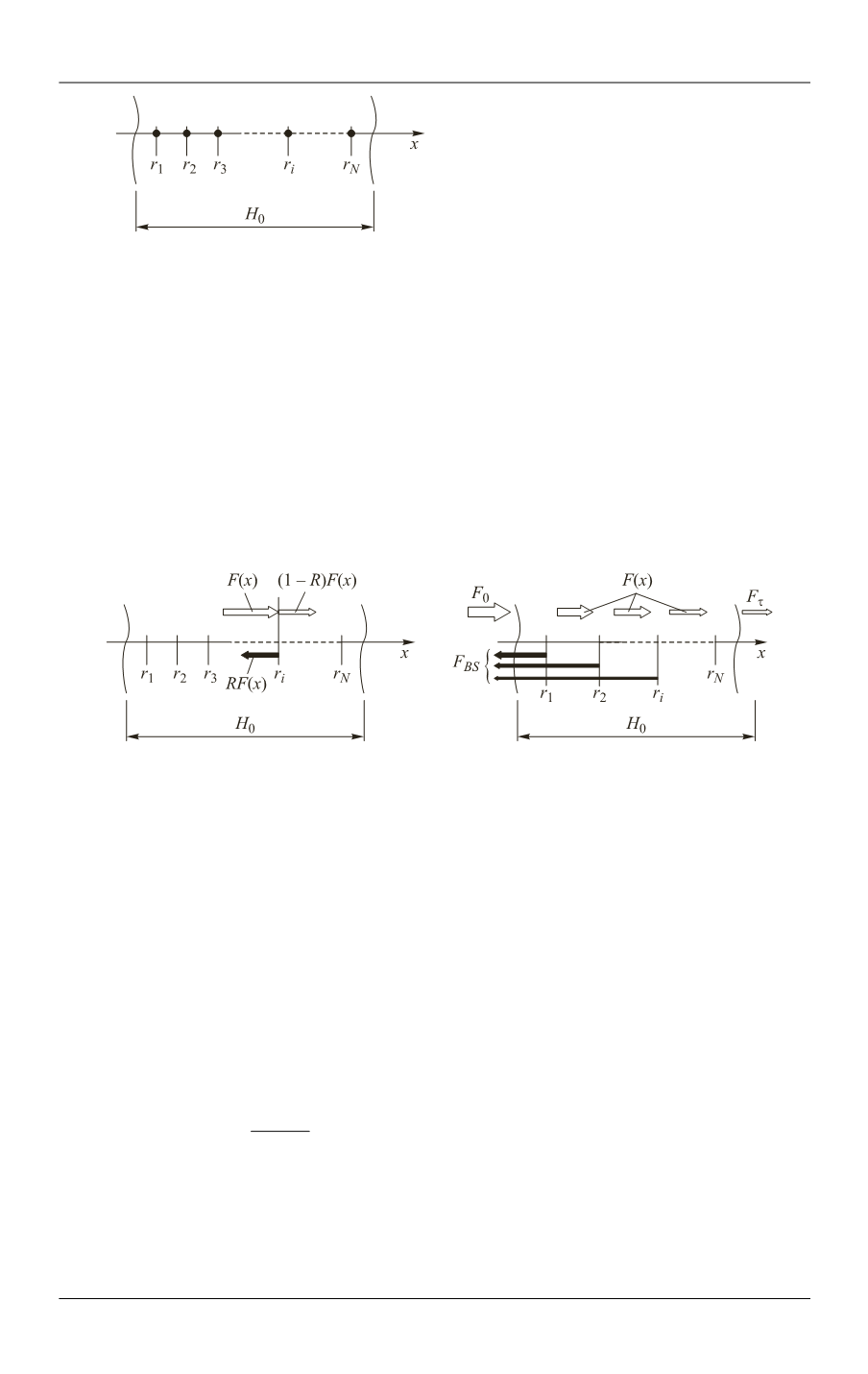
inside the medium. Figure 6 explains the decrement of the flux
F
+
(
x
)
and a formation
of fluxes
F
−
(
x
),
)0( ,
BS
F F
and
0
( ).
F F H
Fig. 6.
Formation of the backscattered and transmitted fluxes in 1D SSA
It is evidently, that in this scheme:
0
0
( )
(1 ) .
N
F F H F R
(13)
Therefore, for each elementary interval Δ
x
, the decrement Δ
F
+
of the propagating
flux
F
+
(
x
) will be equal:
(
) ( )
( )[(1 )
1],
x
F F x x F x F x R
(14)
where
[m
−1
] is the scatterers density inside Δ
x
. One can see that Eq. (14) is
mathematically identical to the Eq. (4), so, applying Eq. (5), it yields:
( )
ln(1 ) ( )
( ),
dF x
R F x SF x
dx
(15)
where by
ln(1 ),
S
R
following KM notations, we denoted the scattering
coefficient. To formulate the increment
ΔF
-
of the propagating flux
F
−
(
x
), we have to
write [15]: